
Quick answer: Excel’s VLOOKUP searches down the first column of a selected table and returns a value from another column on the matching row. For exact product IDs, student IDs or employee numbers, use =VLOOKUP(G2,$A$2:$D$6,3,FALSE). The final FALSE matters: leaving it out requests approximate matching, which can produce incorrect results on unsorted data.
This practical guide uses a small sample table, ten formulas you can copy, error fixes and a comparison with XLOOKUP. Start with the Excel formulas hub and free practice workbook, then explore the free data analysis courses guide to build on these skills.
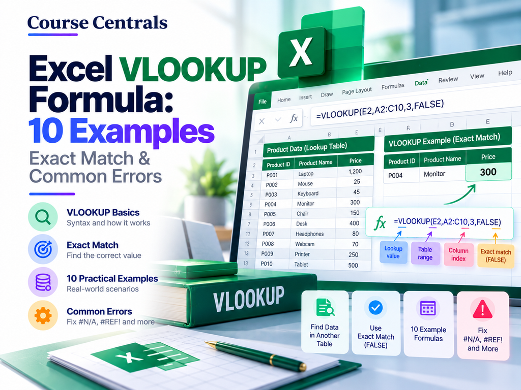
Excel VLOOKUP formula syntax explained
=VLOOKUP(lookup_value,table_array,col_index_num,[range_lookup])
| Argument | What it does | Example |
|---|---|---|
| lookup_value | Value to find | G2 |
| table_array | Lookup table, with key in its first column | $A$2:$D$6 |
| col_index_num | Return-column position within the selected table, starting at 1 | 3 for price |
| range_lookup | FALSE: exact match; TRUE: approximate match | FALSE |
Important: The fourth argument is optional in Excel’s syntax but should not be omitted casually. When omitted, VLOOKUP uses approximate matching. For identifiers, specify FALSE explicitly. For an approximate match with TRUE, sort the first column of the lookup table ascending.
Create the sample dataset
Enter the following values in A1:D6 and type P-103 in cell G2.
| A: SKU | B: Product | C: Price | D: Category |
|---|---|---|---|
| P-101 | Notebook | 15 | Stationery |
| P-102 | Marker | 6 | Stationery |
| P-103 | Mouse | 25 | Electronics |
| P-104 | Headset | 55 | Electronics |
| P-105 | Bottle | 12 | Accessories |
10 VLOOKUP formula examples you can copy
1. Find a product name from its SKU
=VLOOKUP(G2,$A$2:$D$6,2,FALSE)
With P-103 in G2, the result is Mouse. The return column is B, the second column in the selected range.
2. Find a price
=VLOOKUP(G2,$A$2:$D$6,3,FALSE)
Returns 25. This pattern works for price lists and invoice reconciliation.
3. Return a product category
=VLOOKUP(G2,$A$2:$D$6,4,FALSE)
Returns Electronics. The third argument changes to 4 because the category is the fourth column.
4. Type the lookup value directly
=VLOOKUP("P-104",$A$2:$D$6,2,FALSE)
Returns Headset. Literal text values require quotation marks.
5. Show a useful message when an ID is missing
=IFNA(VLOOKUP(G2,$A$2:$D$6,2,FALSE),"SKU not found")
If G2 contains P-999, the formula displays SKU not found. IFNA handles the missing-match error without concealing unrelated formula errors.
6. Match a text prefix with a wildcard
=VLOOKUP("P-10*",$A$2:$D$6,2,FALSE)
Returns the first matching product, Notebook. Wildcards work for text lookup values with exact-match mode, but a broad prefix may match more than one row.
7. Look up a value on another worksheet
=VLOOKUP(G2,Products!$A$2:$D$100,3,FALSE)
Uses a lookup table on a worksheet named Products. Change the sheet name and range to match your workbook.
8. Fill the formula down safely
=VLOOKUP(G2,$A$2:$D$6,3,FALSE)
The dollar signs lock the lookup range. Copying the formula down changes G2 to G3 but preserves the table range.
9. Use approximate matching for score or pricing bands
Create a separate threshold table in J2:K5 with rows 0 Bronze, 100 Silver, 250 Gold, 500 Platinum. Put 300 in H2.
=VLOOKUP(H2,$J$2:$K$5,2,TRUE)
Returns Gold, the tier with the highest threshold that does not exceed 300. The threshold column must be sorted ascending. Never apply this pattern blindly to unsorted identifiers.
10. Find a return column dynamically by its header
=VLOOKUP(G2,$A$1:$D$6,MATCH("Price",$A$1:$D$1,0),FALSE)
MATCH locates the Price header, so you do not need to hard-code the number 3. The lookup key must still occupy the first column of the VLOOKUP table.
VLOOKUP vs XLOOKUP vs INDEX MATCH
| Feature | VLOOKUP | XLOOKUP | INDEX + MATCH |
|---|---|---|---|
| Exact match by default | No | Yes | Specify 0 in MATCH |
| Return value to left of key | Not directly | Yes | Yes |
| Older Excel compatibility | Broad | Not available in all older versions | Broad |
| Return selection | Column number | Separate return array | Separate return range |
Which should you learn? Learn VLOOKUP for maintaining older spreadsheets. For new workbooks on compatible versions, XLOOKUP is often simpler because it can search in either direction and defaults to exact matching. See Microsoft’s XLOOKUP documentation for syntax and version details.
Fix common VLOOKUP errors
| Symptom | Likely cause | Action |
|---|---|---|
| #N/A | No exact match, text-number mismatch, extra spaces | Inspect the key, data type, first column and hidden spaces |
| #REF! | Return column exceeds selected table width | Recount columns from the left of table_array |
| #VALUE! | Invalid argument, including column index below 1 | Review argument values |
| #NAME? | Misspelled function or unquoted text | Check syntax and quotation marks |
| Unexpected result | Approximate match on unsorted data or duplicate keys | Use FALSE for IDs and check uniqueness |
Three rules: specify FALSE for exact identifiers; make sure the lookup key is in the first column of the selected range; and remember that VLOOKUP returns the first matching row, not every match.
Five-minute VLOOKUP practice checklist
- Change G2 to P-105.
- Write formulas returning its name, price and category.
- Replace G2 with P-999.
- Wrap your name lookup with IFNA and display “SKU not found”.
- Compare the exact-match result with an intentionally approximate lookup, then explain the difference.
Expected answers: Bottle, 12, Accessories, SKU not found. Continue with the Course Centrals formula practice workbook, then learn how spreadsheets fit into the wider data analysis learning pathway.
Frequently asked questions
What does the V in VLOOKUP mean?
It means vertical: the function searches down the first column of the table.
Should I use TRUE or FALSE?
Use FALSE for exact identifiers. Use TRUE only for intentional approximate matches on correctly sorted lookup ranges.
Can VLOOKUP search to the left?
Not directly. XLOOKUP or INDEX MATCH is better when the return column sits to the left of the lookup key.
Why does VLOOKUP return #N/A even when a value looks present?
Common causes include text stored as numbers or vice versa, invisible spaces, a lookup range that starts in the wrong column, or an exact key that does not exist.
Is VLOOKUP still worth learning?
Yes. Existing workbooks widely use it, and it remains useful for compatibility with older Excel installations.
Official references and verification
- Microsoft Support: VLOOKUP function
- Microsoft Support: VLOOKUP, INDEX and MATCH
- Microsoft Support: XLOOKUP function
Official documentation checked 15 October 2026. Example data is illustrative. Excel formula argument separators can vary by regional settings.